Image Source: Wikipedia License CC-BY-SA 3.0

If you, like me, frequently commute via public transit, you may be familiar with the following situation:

You arrive at the bus stop, ready to catch your bus: a line that advertises arrivals every 10 minutes. You glance at your watch and note the time... and when the bus finally comes 11 minutes later, you wonder why you always seem to be so unlucky.

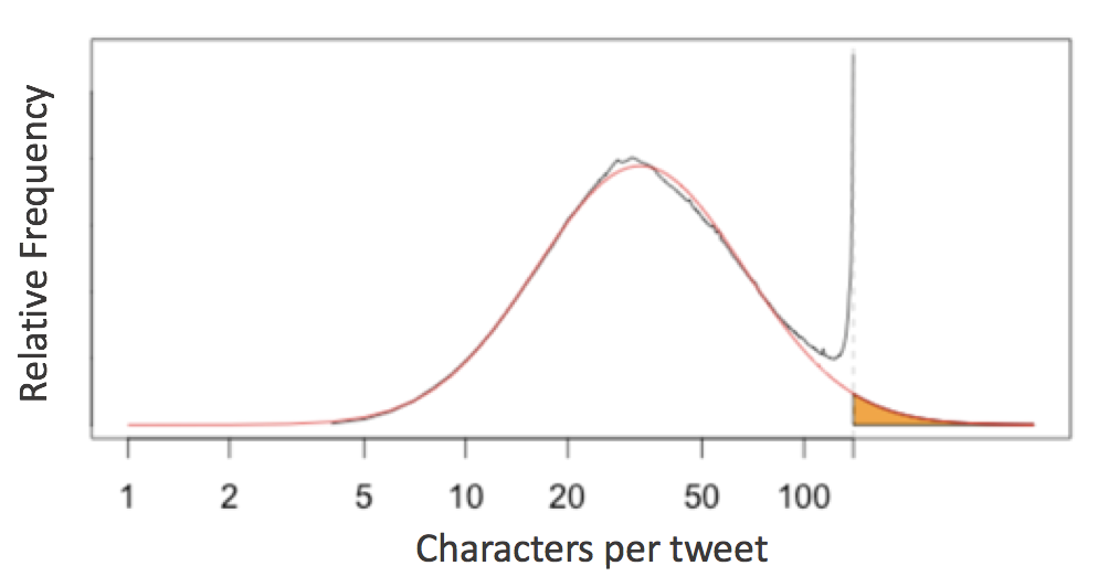
Naïvely, you might expect that if buses are coming every 10 minutes and you arrive at a random time, your average wait would be something like 5 minutes. In reality, though, buses do not arrive exactly on schedule, and so you might wait longer. It turns out that under some reasonable assumptions, you can reach a startling conclusion:

When waiting for a bus that comes on average every 10 minutes, your average waiting time will be 10 minutes.

This is what is sometimes known as the waiting time paradox.

I've encountered this idea before, and always wondered whether it is actually true... how well do those "reasonable assumptions" match reality? This post will explore the waiting time paradox from the standpoint of both simulation and probabilistic arguments, and then take a look at some real bus arrival time data from the city of Seattle to (hopefully) settle the paradox once and for all.

This weekend I found myself in a particularly drawn-out game of Chutes and Ladders with my four-year-old. If you've not had the pleasure of playing it, Chutes and Ladders (also sometimes known as Snakes and Ladders) is a classic kids board game wherein players roll a six-sided die to advance forward through 100 squares, using "ladders" to jump ahead, and avoiding "chutes" that send you backward. It's basically a glorified random walk with visual aids to help you build a narrative. Thrilling. But she's having fun practicing counting, learning to win and lose gracefully, and developing the requisite skills to be a passionate sports fan, so I play along.

On the approximately twenty third game of the morning, as we found ourselves in a near endless cycle of climbing ladders and sliding down chutes, never quite reaching that final square to end the game, I started wondering how much longer the game could last: what is the expected length of a game? How heavy are the tails of the game length distribution? How succinctly could I answer those questions in Python? And then, at some point, it clicked: Chutes and Ladders is memoryless — the effect of a roll depends only on where you are, not where you've been — and so it can be modeled as a Markov process! By the time we (finally) hit square 100, I basically had this blog post written, at least in my head.

When I tweeted about this, people pointed me to a number of similar treatments of Chutes & Ladders, so I'm under no illusion that this idea is original. Think of this as a blog post version of a dad joke: my primary goal is not originality, but self-entertainment, and if anyone else finds it entertaining that's just an added bonus.

Python is quick and easy to code, but can be slow when doing intensive numerical operations. Translating code to Cython can be helpful, but in most cases requires a bit of trial and error to achieve the optimal result. Cython's tutorials contain a lot of information, but for iterative workflows like optimization with Cython, it's often useful to see it done "live".

For that reason, I decided to record some screencasts showing this iterative optimization process, using an Ising Model, as an example application.

In software, it's said that all abstractions are leaky, and this is true for the Jupyter notebook as it is for any other software. I most often see this manifest itself with the following issue:

I installed package X and now I can't import it in the notebook. Help!

This issue is a perrennial source of StackOverflow questions (e.g. this, that, here, there, another, this one, that one, and this... etc.).

Fundamentally the problem is usually rooted in the fact that the Jupyter kernels are disconnected from Jupyter's shell; in other words, the installer points to a different Python version than is being used in the notebook. In the simplest contexts this issue does not arise, but when it does, debugging the problem requires knowledge of the intricacies of the operating system, the intricacies of Python package installation, and the intricacies of Jupyter itself. In other words, the Jupyter notebook, like all abstractions, is leaky.

In the wake of several discussions on this topic with colleagues, some online (exhibit A, exhibit B) and some off, I decided to treat this issue in depth here. This post will address a couple things:

• First, I'll provide a quick, bare-bones answer to the general question, how can I install a Python package so it works with my jupyter notebook, using pip and/or conda?.

• Second, I'll dive into some of the background of exactly what the Jupyter notebook abstraction is doing, how it interacts with the complexities of the operating system, and how you can think about where the "leaks" are, and thus better understand what's happening when things stop working.

• Third, I'll talk about some ideas the community might consider to help smooth-over these issues, including some changes that the Jupyter, Pip, and Conda developers might consider to ease the cognitive load on users.

This post will focus on two approaches to installing Python packages: pip and conda. Other package managers exist (including platform-specific tools like yum, apt, homebrew, etc., as well as cross-platform tools like enstaller), but I'm less familiar with them and won't be remarking on them further.

This week, Twitter upped their single-tweet character limit from 140 to 280, purportedly based on this interesting analysis of tweet lengths published on Twitter's engineering blog. The gist of the analysis is this: English language tweets display a roughly log-normal distribution of character counts, except near the 140-character limit, at which the distribution spikes:

The analysis takes this as evidence that twitter users often "cram" their longer thoughts into the 140 character limit, and suggest that a 280-character limit would more naturally accommodate the distribution of people's desired tweet lengths.

This immediately brought to mind another character limit that many Python programmers face in their day-to-day lives: the 79-character line limit suggested by Python's PEP8 style guide:

Limit all lines to a maximum of 79 characters.

I began to wonder whether popular Python packages (e.g. NumPy, SciPy, Pandas, Scikit-Learn, Matplotlib, AstroPy) display anything similar to what is seen in the distribution of tweet lengths.

Spoiler alert: they do! And the details of the distribution reveal some insights into the programming habits and stylistic conventions of the communities who write them.

I just got home from my sixth PyCon, and it was wonderful as usual. If you weren't able to attend—or even if you were—you'll find a wealth of entertaining and informative talks on the PyCon 2017 YouTube channel.

Two of my favorites this year were a complementary pair of talks on Python dictionaries by two PyCon regulars: Raymond Hettinger's Modern Python Dictionaries A confluence of a dozen great ideas and Brandon Rhodes' The Dictionary Even Mightier (a followup of his PyCon 2010 talk, The Mighty Dictionary)

Raymond's is a fascinating dive into the guts of the CPython dict implementation, while Brandon's focuses more on recent improvements in the dict's user-facing API. One piece both mention is the addition in Python 3.6 of a private dictionary version to aid CPython optimization efforts. In Brandon's words:

"PEP509 added a private version number... every dictionary has a version number, and elsewhere in memory a master version counter. And when you go and change a dictionary the master counter is incremented from a million to a million and one, and that value a million and one is written into the version number of that dictionary. So what this means is that you can come back later and know if it's been modified, without reading maybe its hundreds of keys and values: you just look and see if the version has increased since the last time you were there."

He later went on to say,

"[The version number] is internal; I haven't seen an interface for users to get to it..."

which, of course, I saw as an implicit challenge. So let's expose it!

This week I published the preprint of a manuscript that started as a blog post, but quickly out-grew this medium: Understanding the Lomb-Scargle Periodogram.

Figure 24 from Understanding the Lomb-Scargle Periodogram. The figure shows the true period vs the periodogram peak for a simulated dataset with an observing cadence typical of ground-based optical astronomy. The simulation reveals common patterns of failure of the Lomb-Scargle method that are not often discussed explicitly, but are straightforward to explain based on the intuition developed in the paper; see Section 7.2 for a detailed discussion.

Over the last couple years I've written a number of Python implementations of the Lomb-Scargle periodogram (I'd recommend AstroPy's LombScargle in most cases today), and also wrote a marginally popular blog post and somewhat pedagogical paper on the subject. This all has led to a steady trickle of emails from students and researchers asking for advice on applying and interpreting the Lomb-Scargle algorithm, particularly for astronomical data. I noticed that these queries tended to repeat many of the same questions and express some similar misconceptions, and this paper is my attempt to address those once and for all — in a "mere" 55 pages (which includes 26 figures and 4 full pages of references, so it's not all that bad).

I've found one of the best ways to grow in my scientific coding is to spend time comparing the efficiency of various approaches to implementing particular algorithms that I find useful, in order to build an intuition of the performance of the building blocks of the scientific Python ecosystem.

In this vein, today I want to take a look at an operation that is in many ways fundamental to data-driven exploration: the group-by, otherwise known as the split-apply-combine pattern. An architypical example of a summation group-by is shown in this figure, borrowed from the Aggregation and Grouping section of the Python Data Science Handbook:

The basic idea is to split the data into groups based on some value, apply a particular operation to the subset of data within each group (often an aggregation), and then combine the results into an output dataframe. Python users generally turn to the Pandas library for this type of operation, where it is is implemented effiently via a concise object-oriented API:

Earlier this week a tweet made the rounds which features a video that nicely demonstrates chaotic dynamical systems in action:

A visualization of chaos: 41 triple pendulums with very slightly different initial conditions pic.twitter.com/CTiABFVWHW

— Fermat's Library (@fermatslibrary) March 5, 2017

Edit: a reader pointed out that the original creator of this animation posted it on reddit in 2016.

Naturally, I immediately wondered whether I could reproduce this simlulation in Python. This post is the result.

Jupyter notebooks provide a useful environment for interactive exploration of data. A common question I get, though, is how you can progress from this nonlinear, interactive, trial-and-error style of exploration to a more linear and reproducible analysis based on organized, packaged, and tested code. This series of videos presents a case study in how I personally approach reproducible data analysis within the Jupyter notebook.

Each video is approximately 5-8 minutes; the videos are available in a YouTube Playlist. Alternatively, below you can find the videos with some description and links to relevant resources