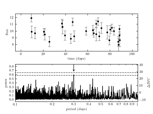Image source: astroML. Source code here

Edit, Spring 2017: For an in-depth guide to the practical use of Lomb-Scargle periodograms, see the paper discussed in A Practical Guide to the Lomb-Scargle Periodogram.

Edit, Summer 2016: All of the implementations discussed below have been added to AstroPy as of Version 1.2, along with logic to choose the optimal implementation automatically. Read more here: astropy.stats.LombScargle.

The Lomb-Scargle periodogram (named for Lomb (1976) and Scargle (1982)) is a classic method for finding periodicity in irregularly-sampled data. It is in many ways analogous to the more familiar Fourier Power Spectral Density (PSD) often used for detecting periodicity in regularly-sampled data.

Despite the importance of this method, until recently there have not been any (in my opinion) solid implementations of the algorithm available for easy use in Python. That has changed with the introduction of the gatspy package, which I recently released. In this post, I will compare several available Python implementations of the Lomb-Scargle periodogram, and discuss some of the considerations required when using it to analyze data.

To cut to the chase, I'd recommend using the gatspy package for Lomb-Scargle periodograms in Python, and particularly its gatspy.periodic.LombScargleFast algorithm which implements an efficient pure-Python version of Press & Rybicki's $O[N\log N]$ periodogram. Below, I'll dive into the reasons for this recommendation.

Example: Lomb-Scargle on Variable Stars¶

As an motivation, let's briefly consider some data from my own field: observations of an RR Lyrae-type variable star. RR Lyrae are small stars – about 50% the mass of our sun – which pulsate with a regular period on order half a day. Their relatively consistent peak intrinsic brightness allows for an accurate estimation of their distance from the sun, and thus they are important for studies such as understanding the substructure of the Milky Way galaxy. Because of this and other similar applications, detecting the telltale periodic variation of RR Lyrae stars within noisy data is an important statistical task for astronomers.

Here we will quickly demonstrate what this looks like in practice, using tools from the astroML package to download some data, and tools from the gatspy package to detect the periodicity.

We'll start with some typical Python import statements:

Now we'll download some data from the LINEAR dataset, using tools in astroML. We'll plot the data to see what we're working with:

This data has around 250 observations spread across about 2000 days, and we're hoping to detect a period of order 0.5 days. If the series were regularly-sampled, we'd be far above the Nyquist limit and all hope would be lost. Fortunately for astronomers, the assumptions behind the Nyquist sampling limit do not hold for irregular sampling rates, and we can proceed with no problem.

Let's start by computing and plotting the Lomb-Scargle Periodogram for this data, using tools from gatspy:

The periodogram gives a measure of periodic content as a function of period; we see here a strong peak at around 0.61 days. Other lower peaks are due to some combination of higher-order harmonics in the data and effects of the irregular survey window. While we could find this maximum manually from the above grid, gatspy provides a better way: a built-in two-stage grid-search that accurately determines the best period in a specified range:

We see that the optimizer determined that it needed a grid of over 40,000 points to adequately cover the frequency grid (more on this below), and in the end arrived at a best period of 0.6105 days. Given this detected period, we can fold the input data and over-plot a best-fit empirical RR Lyrae template to see the fit:

This very close template fit gives a strong indication that the star in question is an RR Lyrae.

Computational Considerations for Lomb-Scargle¶

The Lomb-Scargle periodogram involves the computation of a power $P(\omega)$ at a set of frequencies $\omega_i$. For data $\{y_k\}$ pre-centered such that $\sum_k y_k = 0$, the expression for the power is:

$$ P(\omega) \propto \frac{\left[\sum_k y_k \cos\omega(t_k - \tau)\right]^2} {\sum_k \cos^2\omega(t_k - \tau)} + \frac{\left[\sum_k y_k \sin\omega(t_k - \tau)\right]^2} {\sum_k \sin^2\omega(t_k - \tau)} $$

where $\tau$ is an easily computed time-offset which orthogonalizes the model and makes $P(\omega)$ independent of a translation in $t$.

Rather than get lost in the math, I want to emphasize the key feature of this expression: for any frequency $\omega$, the power is an $O[N]$ computation involving simple trigonometric sums over the data, where $N$ is the number of observed data points. The main computational question then becomes: how many frequencies must you compute? In my experience, the most common mistake people make when doing this sort of periodic analysis is not thinking hard enough about the frequency grid. It turns out that the grid-spacing question is very important. If you choose too fine a grid, you do much more computation than is required. Worse, if you choose too coarse a grid, the periodogram peak may fall between grid points and you'll miss it entirely!

Let's think about the required frequency range and frequency spacing for Lomb-Scargle.

Frequency spacing¶

First we'll choose the spacing of the frequency grid. If you're asking about a candidate frequency $f$, then data with range $T = t_{max} - t_{min}$ contains $T \cdot f$ complete cycles. If our error in frequency is $\delta f$, then $T\cdot\delta f$ is the error in number of cycles between the endpoints of the data. It's clear that this error must not be a significant fraction of a cycle, or the fit could be drastically affected. This leads to an approximate grid-spacing criterion:

$$ T\cdot\delta f \ll 1 $$

Commonly, we'll choose some oversampling factor (say, 5) and use $\delta f = (5T)^{-1}$ as our frequency grid spacing.

Frequency limits¶

Next, we need to choose the upper and lower limits of the frequency grid. On the low end, $f=0$ is suitable, but causes some numerical problems – we'll go one step away and use $\delta f$ as our minimum frequency. But on the high end, we need to make a choice: what's the highest frequency we'd trust our data to be sensitive to? At this point, many people are tempted to mis-apply the Nyquist-Shannon sampling theorem, and choose some version of the Nyquist limit for the data (based on, say, the minimum or mean spacing between observations). But this is entirely wrong! The Nyquist frequency is derived from special properties of regularly-sampled data, and does not apply – even approximately – to irregularly-sampled time-series. In fact, as we saw above, irregularly-sampled data can be sensitive to much, much higher frequencies than even the minimum spacing between observations. With this in mind, the upper limit for frequencies should be determined based on what kind of signal you are looking for.

Still, a common (if dubious) rule-of-thumb is that the high frequency is some multiple of what Press & Rybicki call the "average" Nyquist frequency,

$$ \hat{f}_{Ny} = \frac{N}{2T} $$

This means that the "typical" number of frequencies you'll need is

$$ N_{freq} \sim O\left[\frac{\hat{f}_{Ny}}{\delta f}\right] \sim O\left[\frac{N/(2T)}{1/T}\right] \sim O[N] $$

That is, the number of frequencies to search will scale with the number of data points!

Computational Complexity¶

From the above considerations, we see that the determination of the optimal Lomb-Scargle period within $N$ points requires computing an $O[N]$ expression for power across $O[N]$ grid points; that is, Lomb-Scargle is naively an $O[N^2]$ algorithm.

This computational complexity can be improved in one of several ways. Most notably, in a 1989 paper, Press and Rybicki proposed a clever method whereby a Fast Fourier Transform is used on a grid extirpolated from the original data, such that this naively $O[N^2]$ problem can be solved in $O[N\log N]$ time. The broad idea is that when you compute sums of sines and cosines for one frequency, this gives you some amount of information about those sums computed at another frequency, and by carefully using all information across a frequency grid, you can significantly reduce the number of required operations.

Thus the fundamental divide between Lomb-Scargle implementations is whether they use the naive $O[N^2]$ algorithm or the $O[N\log N]$ algorithm of Press & Rybicki and other similar approaches.

Lomb-Scargle Algorithms in Python¶

Now we get to the meat of this post: Lomb-Scargle implementations written in Python. If you search this on Google, you'll currently find links to several available implementations. Here I'm going to delve into and compare the following four implementations:

• scipy.signal.lombscargle, an $O[N^2]$ implementation from SciPy.
• astroML.time_series.lomb_scargle, an $O[N^2]$ implementation from astroML.
• gatspy.periodic.LombScargle, an $O[N^2]$ implementation from gatspy.
• gatspy.periodic.LombScargleFast, an $O[N\log N]$ implementation, also from gatspy.

Let's see some examples of the above tools:

scipy.signal.lombscargle¶

The SciPy Lomb-Scargle periodogram is a C implementation of the naive $O[N^2]$ algorithm. The algorithm cannot account for noise in the data, and has some other quirks as well:

• it requires you to center your data (by subtracting the mean) before computing the periodogram. If you do not, the results will be garbage.
• it computes the unnormalized periodogram, which can be normalized manually as we'll see below.
• it takes angular frequencies as the argument.

Let's use scipy's algorithm to plot the periodogram of the data shown above. Note that the results will not be identical, because this algorithm ignores the noise in the data and doesn't fit for the data mean.

Against the above recommendations, we'll choose a simple regular grid in period for the plot:

Comparing to the first periodogram plot, we see that becuase our period grid here is too coarse at low frequencies, some of the peak structure is missed by this visualization. Consider this a warning against arbitrarily choosing a period gridding!

astroML.time_series.lomb_scargle¶

AstroML has two $O[N^2]$ implementations of Lomb-Scargle: one in astroML and one in astroML_addons, which is a collection of C extensions which replace slower functionality in the pure-python astroML package. In order to use the faster version, make sure you install both packages; e.g.

$ pip install astroML
$ pip install astroML_addons

Some important features of astroML's Lomb Scargle periodogram:

• unlike scipy, it uses an extended periodogram model which can correctly account for uncorrelated Gaussian measurement error.
• like scipy, it takes angular frequencies as its argument.
• unlike scipy, it implements a floating mean periodogram, meaning that the data centering required for scipy is not required here, but it goes beyond simple centering: the mean of the data is fit as part of the model, which has advantages in many real-world scenarios. To directly compare to scipy's standard Lomb Scargle pass generalized=False.

Let's repeat the above plot with this periodogram:

gatspy.periodic.LombScargle¶

Gatspy's basic Lomb-Scargle algorithm is an $O[N^2]$ implementation, but is implemented differently than either of the above versions. It uses a direct linear algebra approach which carries some additional computational and memory overhead. The reason for this approach is that it naturally accommodates several extensions to the periodogram, including floating mean, multiple terms, regularization, and multi-band models (more details in VanderPlas & Ivezic (2015), the paper that inspired gatspy).

Gatspy is a pure python package, and thus installation is easy and requires no compilation of C or Fortran code:

$ pip install gatspy

Some important features of this implementation:

• like astroML, it uses an extended periodogram model which correctly accounts for uncorrelated Gaussian measurement error.
• unlike astroML, it takes periods as its argument.
• like astroML, it uses a floating mean model by default. To compare directly to scipy's non-floating-mean model, set fit_offset=False.
• it has an API inspired by scikit-learn, where the model itself is a class instance, the model is applied to data with a fit() method, and the periodogram is computed via a score() method.

Let's repeat the above periodogram using this tool:

gatspy.periodic.LombScargleFast¶

Gatspy's fast Lomb-Scargle is an $O[N\log N]$ algorithm built on a pure Python/numpy implementation of the Press & Rybicki FFT/extirpolation method. Note that a requirement of this fast algorithm is that it be computed on a regular grid of frequencies (not periods), and so to attain this performance it provides the score_frequency_grid() method which takes 3 arguments: the minimum frequency f0, the frequency spacing df, and the number of grid points N.

Some features of the model

• like astroML, it uses an extended periodogram model which correctly accounts for uncorrelated Gaussian measurement error.
• it takes a regular frequency grid as its argument for the fast computation; note that the score() function itself falls back on the slower LombScargle approach above.
• like astroML, it uses a floating mean model by default. To compare directly to scipy, set fit_offset=False.
• it has an identical API to the LombScargle object above.

Let's take a look at computing the periodogram:

You'll notice here that this approach shows a lot more high-frequency peaks than any of the above versions. This is not because it is computing a different model; it is because we are using a finer frequency grid which does not miss these peaks. The above versions, with a regular grid of 4000 periods miss these important features, and give the user absolutely no warning that these features are missed! Keep this in mind as you choose grid parameters while following the above discussion.

If you want to make sure you're using a sufficient grid, you can use the periodogram_auto() method of LombScargleFast, which computes a sufficient frequency grid for you using the rules-of-thumb discussed in the previous section:

The model decided that we needed over 100,000 periods, between about 0.1 days (which was tuned by the nyquist_factor argument) and about 10,000 days (which is derived from the time-span of the data). Plotting the results as above, we see a similar periodogram:

The LombScargleFast algorithm computes these $10^5$ periodogram steps very quickly; I wouldn't suggest any of the other methods with a grid of this size!

Benchmarking Lomb-Scargle Implementations¶

As a final piece of the picture, let's compare the execution speed of the four approaches. We can do this with IPython's %timeit magic function using the following script. Note that this script will take several minutes to run, as it automatically does multiple passes of each benchmark to minimize system timing variation. For efficiency, we cut-off the slower algorithms at high $N$:

When these timings are finished, we can plot the results to get an idea of how the algorithms compare:

Each model has a characteristic performance curve:

• The scipy and astroML algorithms show similar behavior: fast $O[1]$ scaling at the small-$N$ limit, and clear $O[N^2]$ scaling at the large-$N$ limit. SciPy is slightly faster, primarily due to the fact that it computes the simpler noiseless non-floating-mean model.
• Gatspy's LombScargle also becomes $O[N^2]$ at large $N$, but is dominated at small $N$ by an $O[N]$ contribution which comes from allocating & building the matrices associated with its linear algebraic approach. As $N$ grows larger than $\sim 10^4$, however, gatspy's model begins to beat the performance of the other two $O[N^2]$ algorithms.
• Gatspy's LombScargleFast has an upfront $O[1]$ cost that makes it slower than other approaches at small $N$, but as $N$ grows its $O[N\log N]$ scaling means it dominates the performance of the other approaches by orders of magnitude.

If you'd like to push the speed of the computation even further, there may be some options available. For example, the pynfftls package implements an $O[N\log N]$ Lomb-Scargle based on the NFFT algorithm, which is similar to the NUFFT that I discussed in a previous post. The pynfftls installation depends on prior installations of the NFFT and FFTW libraries. These libraries are best-in-class implementations of their respective algorithms, and from my past experience with them, I'd expect pynfftls to be around a factor of 10 faster than LombScargleFast with the same $O[N\log N]$ scaling.

I should mention that I briefly tried installing pynfftls for this post, but ran into difficulties with linking the source to the appropriate C headers and library/shared object files. No doubt with a couple hours of tinkering it could be done, but in a conda world I've found my threshold of tolerance for such installation headaches has gone way down. Package developers take note: in most situations, ease of installation is easily worth a factor of a few in runtime performance. If any readers want to tackle the comparison between LombScargleFast and pynfftls, I'd be intrested to learn whether my factor-of-ten intuition is correct!

Conclusion¶

If there's anything I want you to take from the above discussion, it's these three points:

• Naive application of Nyquist-style limits to irregularly-sampled data is 100% wrong. Don't be the next person to make this mistake in the published literature! I've been meaning to write a full rant/post on this subject for a while. Perhaps I will someday.
• Selection of period/frequency grids for Lomb-Scargle analysis should not be taken lightly. It's very easy to inadvertently use too coarse of a grid, and entirely miss important periodogram peaks!
• Use gatspy.periodic.LombScargleFast if you want any easy-to-install means of computing a fast, $O[N\log N]$ Lomb-Scargle periodogram in Python.

This post was written entirely in the IPython notebook. You can download this notebook, or see a static view here.